Product pricing in (simulated) Moonlighter with Bayesian bandits to maximize customer sadness

I played Moonlighter a while ago and really enjoyed it. The combination of running a shop during the day and combing through dungeons at night (hence "moonlighter") to find items to sell in said shop or craft weapons/potions was one of the more refreshing gameplay loops I'd encountered in a while.

At some point I learned about a method called Bayesian bandits and thought it might be a good approach for deciding what items to sell and for how much in my in-game store.

What is Moonlighter?

Moonlighter is a video game where the core game loop revolves around obtaining items in dungeons at night and selling those items in your shop during the day.

Your shop has a limited, though upgradable, number of shelves where you can place items and set their price. After you open up, customers randomly look at items and decide whether to buy based on their willingness to pay that amount. The customer shows one of four emotions when doing this (my labels):

1. Ecstatic: item is underpriced
2. Content: item is priced just right
3. Sad: item is overpriced but they will still buy it, though its popularity and, hence, the future price all customers are willing to pay will go down temporarily (expiring bad Yelp review?)
4. Angry: item is overpriced so they will not buy it

Therefore, making the customer content (instead of sad) AND making the most money is incentivized.

Potential prices have a huge range of 0 to 9999999. To help players get started with pricing, acquired items are placed in a ledger, from highest to lowest price, and in sections with clearly marked lower and upper bounds. For instance, ancient pots are indicated to have a price somewhere between 2 and 275 gold.

This is a limited simulation of Moonlighter's shop mechanic

I started out with an ambitious plan to build a tool for users to price their items in the actual game. However, at some point I realized that this would require the user to constantly note the popularity of every single inventory item any time a new item had to be placed on a shelf, which sounds like a terrible user experience.

I considered writing some sort of mod for the game but didn't feel like learning C#. It looked like the only way forward was to simulate customer reactions myself and turn this project into an article instead of a neat web app where I get to fiddle with htmx :(

Other than price, customer reactions in Moonlighter are affected by customer type (e.g. regular, rich, etc), item popularity (i.e. regular, low, high), whether it's in a display case or not, and possibly others. To simplify my version, I decided to only consider the case where popularity and customer/shelf types are normal. Since popularity is eliminated as a factor, this version doesn't include a lowering of generally acceptable price upon a sad customer reaction.

What this boils down to is, customers don't buy if they are angry and buy otherwise. Hence, the optimal scenario is to just maximize the price, in which case they end up sad.

Bayesian bandits algorithm

I don't intend this article to be a primer on Bayesian bandits. I learned from this section of Think Bayes 2.

The essential algorithm is to keep an updated understanding of the probability of rewards (i.e. a posterior distribution) for different options as new data is encountered. Then when a choice is to be made between them, sample a value from each option's distribution and use the option with the highest value (i.e. Thompson Sampling). Finally, update your understanding of the reward distributions with the result and continue the cycle until some stopping criteria (e.g. out of items to sell).

For this simulation, the algorithm keeps track of distributions consisting of the probability that a particular price is the ideal/highest price for every item. For this simplified version of the shop mechanic, the probabilities of each price are all equal unless they are zero because they are outside particular lower and upper bounds. These bounds are initially determined by the ledger bounds mentioned earlier. The bounds are updated by the simulated customer reactions, as described below.

This process ended up being equivalent to a Bayesian update, whereby the probability distribution of each reaction at each ideal item price (i.e. the likelihood) is generated then multiplied by the current probabilities of ideal item prices (i.e. the posterior or, at the beginning, prior). Hence, to simplify things I just went with the manual update of the price bounds.

Technology and data used

I used SQLite to keep track of my inventory, shelves, customer reactions, and the bounds for item prices and Python to interact with it and facilitate the Bayesian bandits algorithm.

Here's the function, containing the initialization query (DDL), I used to initialize the tables:

  
    def initialize_database():
        execute_sqlite_script(
            """
            pragma foreign_keys = on;

            /* Bounds used to simulate customer reactions to prices */
            create table if not exists price_reaction_bounds (
                item text not null,
                cheap_upper integer not null,
                perfect_upper integer not null,
                expensive_upper integer not null
            ) strict;

            create table if not exists allowed_moods (
                mood text primary key
            ) strict;
            insert or ignore into allowed_moods(mood) values
                ('ecstatic'),
                ('content'),
                ('sad'),
                ('angry');

            create table if not exists reactions (
                shelf_id integer not null,
                item text not null,
                price integer not null,
                mood text not null,
                foreign key (mood) references allowed_moods(mood)
            ) strict;
            create table if not exists thompson_competitions (
                competition_ind integer not null,
                item text not null,
                price_lower_bound integer not null,
                price_upper_bound integer not null,
                sampled_price integer not null
            ) strict;
            create table if not exists price_bound_history (
                reaction_id integer,
                item text not null,
                low integer not null,
                high integer not null
            ) strict;
            create table if not exists inventory (
                item text not null,
                count integer not null
            ) strict;
            create table if not exists inventory_changes (
                item text not null,
                change integer not null
            ) strict;
            create table if not exists shelves (
                id integer not null,
                item text,
                price integer
            ) strict;
            create table if not exists shelf_history (
                shelf_id integer not null,
                item text,
                price integer
            ) strict;
            """)

  

Inventory is kept track of via the inventory and inventory_changes table. Whenever I add or remove an item from it I note a positive or negative count change in the inventory_changes table and use it to rebuild the inventory table. Shelves, their items, and prices are kept track of in the shelf_history table. The current state of the shelves is kept in the shelves table. The moods customers display in reaction to items and their prices is kept in the reactions table, along with the id of the shelf where it occurred. Understanding of what the potential best price is for an item is kept in the price_bound_history table. The prices sampled from item price bounds, in the Thompson sampling process, are kept in the thompson_competitions table. Lower and upper prices for different customer moods from the official Moonlighter wiki, used to simulate customer reactions to prices, are kept in the price_reaction_bounds table. Finally, I included an allowed_moods table containing all unique moods as a check (i.e. foreign key constraint) on other tables to prevent adding something other than the 4 described above.

How the simulation works

Here's the main code that runs the simulation:

  
    clear_database()
    initialize_database()
    initialize_shelves(shelf_count=4)
    item_count = 20
    add_items_2_inventory(
        item_counts={
            'gold_runes': item_count,
            'broken_sword': item_count,
            'vine': item_count,
            'root': item_count,
            'hardened_steel': item_count,
            'glass_lenses': item_count,
            'teeth_stone': item_count,
            'iron_bar': item_count,
            'crystallized_energy': item_count,
            'golem_core': item_count})
    initialize_price_bound_history({
        '275|3000': [
            'gold_runes', 'hardened_steel'],
        '2|275': [
            'broken_sword', 'ancient_pot', 'crystallized_energy',
            'glass_lenses', 'golem_core', 'iron_bar', 'root', 'teeth_stone', 'vine']})
    add_price_reaction_bounds(
        price_reaction_bounds=(
            pd.DataFrame(
                [
                    ['broken_sword', 134, 165, 173],
                    ['crystallized_energy', 89, 110, 115],
                    ['glass_lenses', 89, 110, 115],
                    ['gold_runes', 269, 330, 345],
                    ['golem_core', 89, 110, 115],
                    ['hardened_steel', 269, 330, 345],
                    ['iron_bar', 21, 28, 30],
                    ['root', 3, 6, 8],
                    ['teeth_stone', 3, 6, 8],
                    ['vine', 0, 3, 5]],
                columns=[
                    'item', 'cheap_upper', 'perfect_upper',
                    'expensive_upper'])
            .to_dict('records')))
    rng = np.random.default_rng(71071763)
    fill_empty_shelves_w_priced_items(rng)
    inventory_item_count = get_inventory_item_count()
    shelf_item_count = get_shelf_item_count()
    while inventory_item_count or shelf_item_count:
        shelf_reaction = get_random_shelf_reaction(rng)
        record_reaction(
            shelf_id=shelf_reaction['shelf_id'],
            mood=shelf_reaction['mood'])
        update_price_bound_history()
        if shelf_reaction['mood'] == 'angry':
            add_items_2_inventory(
                item_counts={
                    get_shelf_item_and_price(shelf_id=shelf_reaction['shelf_id'])['item']: 1})
        empty_shelf(shelf_id=shelf_reaction['shelf_id'])
        fill_empty_shelves_w_priced_items(rng)
        replace_items_on_shelf_violating_price_bounds()
        inventory_item_count = get_inventory_item_count()
        shelf_item_count = get_shelf_item_count()

  

I start by clearing all tables from the SQLite database. Then I initialize the database with the tables discussed above and add rows for each shelf in the shop. In this case, I initialize with only 4 shelves, since that is what you have at the beginning of the game. Next I initialize my inventory with 20 of each item. The mix of items (e.g. crystallized energy, root, etc) are what I obtained in an initial run through the first dungeon. Then I add the lower and upper bounds for each of those items dictated in the ledger and add the bounds used to simulate customer reactions. At this point all of the data we need to start the simulation has been populated.

We start by filling all 4 empty shelves with items from the inventory at their corresponding prices, both determined by Thompson sampling. The way this works is, a price from the lower to the upper bounds for each item is randomly chosen and the item with the highest price is used at that price on the shelf. As described earlier, these bounds represent the algorithm's understanding of the range of prices the ideal/highest/best price is in for that item.

Once all of the shelves are full, the simulation goes through multiple rounds of these steps:

1. A customer reacts to a random shelf's item/price, which is recorded
2. The item price bound distributions are updated based on the reaction
3. The item is removed from the shelf and is added to the inventory only if the customer is angry, since they didn't buy it
4. The empty shelf is filled with another item/price determined by Thompson sampling
5. Shelves with items whose prices are outside of the current item price bounds are replaced using items/prices determined by Thompson sampling

This process continues until both the inventory and shelves are empty.

Regarding the item price bounds update upon a customer reaction, if the reaction to an item and its price is angry and the bounds don't match the upper bound is set to the price minus 1 gold, otherwise it is kept the same. If the mood is content or ecstatic the lower bound is set to the price plus 1 gold. If the mood is sad and bounds don't match then the lower bound is set to just the price. The reason for this is, we don't want to risk making the lower bound higher than the upper bound in the scenario where the bounds match. If the mood is sad and the bounds do match then the lower bound remains unchanged.

Here is the corresponding Github repository in case you're interested in running the simulation yourself.

Simulation results

Here's the inventory count of each item as the simulation progresses:

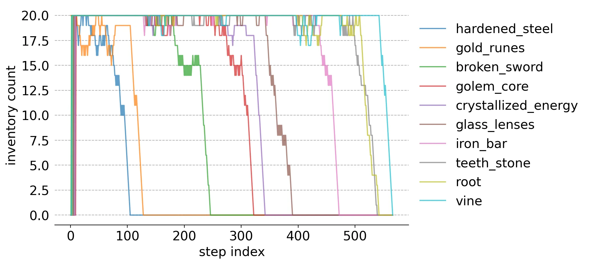
The item depletion order was:

1. hardened steel
2. gold runes
3. broken sword
4. golem core
5. crystallized energy
6. glass lenses
7. iron bar
8. teeth stone
9. root
10. vine

One caveat to this ordering is the algorithm switched focus from selling teeth stone to selling roots around step 525 and switched again soon after.

Here are the final and ideal (i.e. highest while sad and not angry) prices for all items:

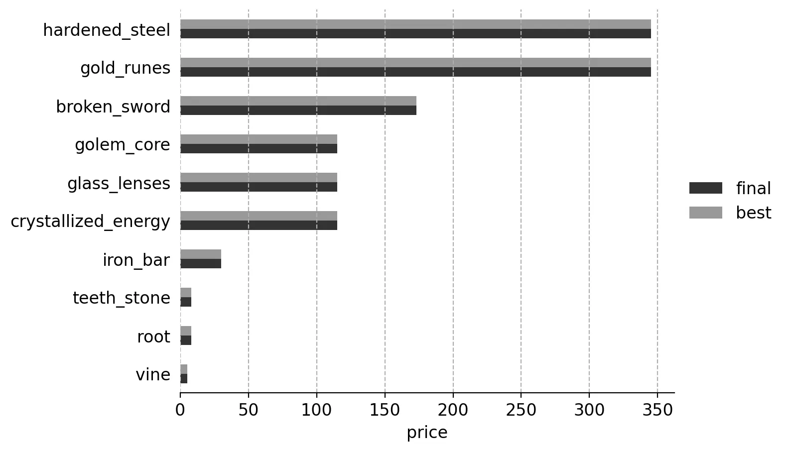
The algorithm converged on the best prices!

The depletion order makes a lot of sense given this graph. The Bayesian bandits algorithm identified groups corresponding to the same ideal price and sold them off in order from highest to lowest price.

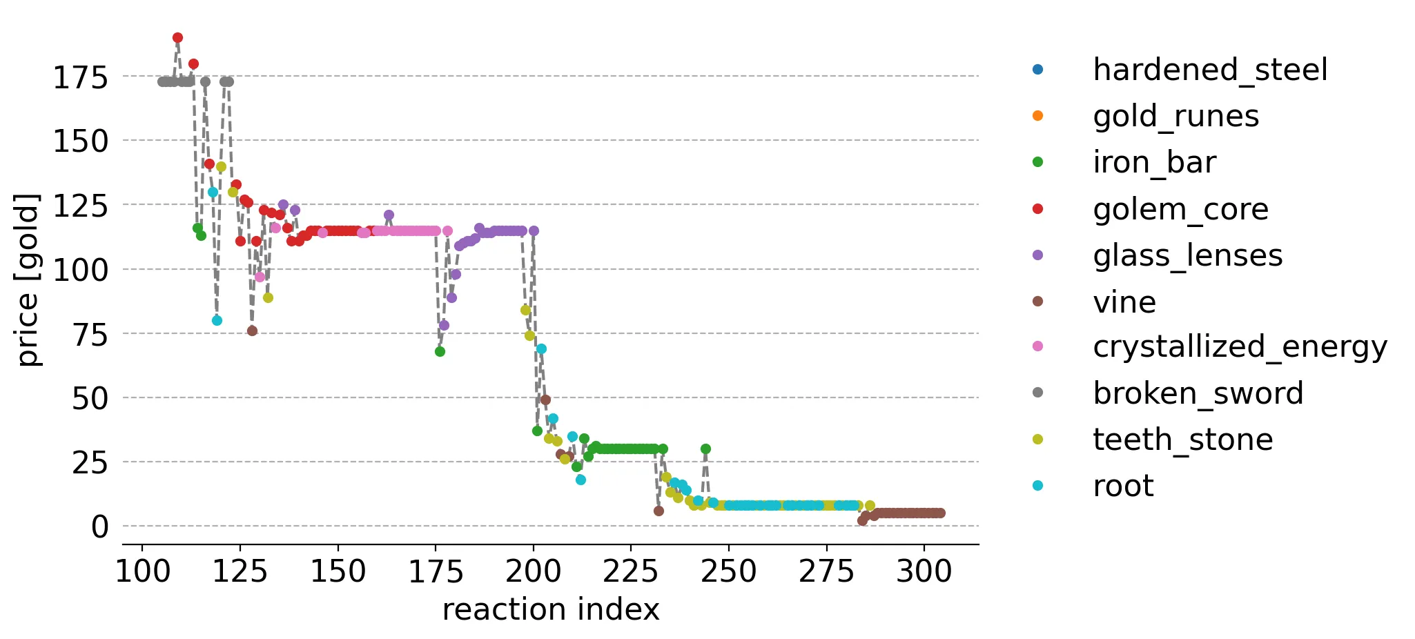
For another view, here are the items and prices for the first 100 customer reactions:

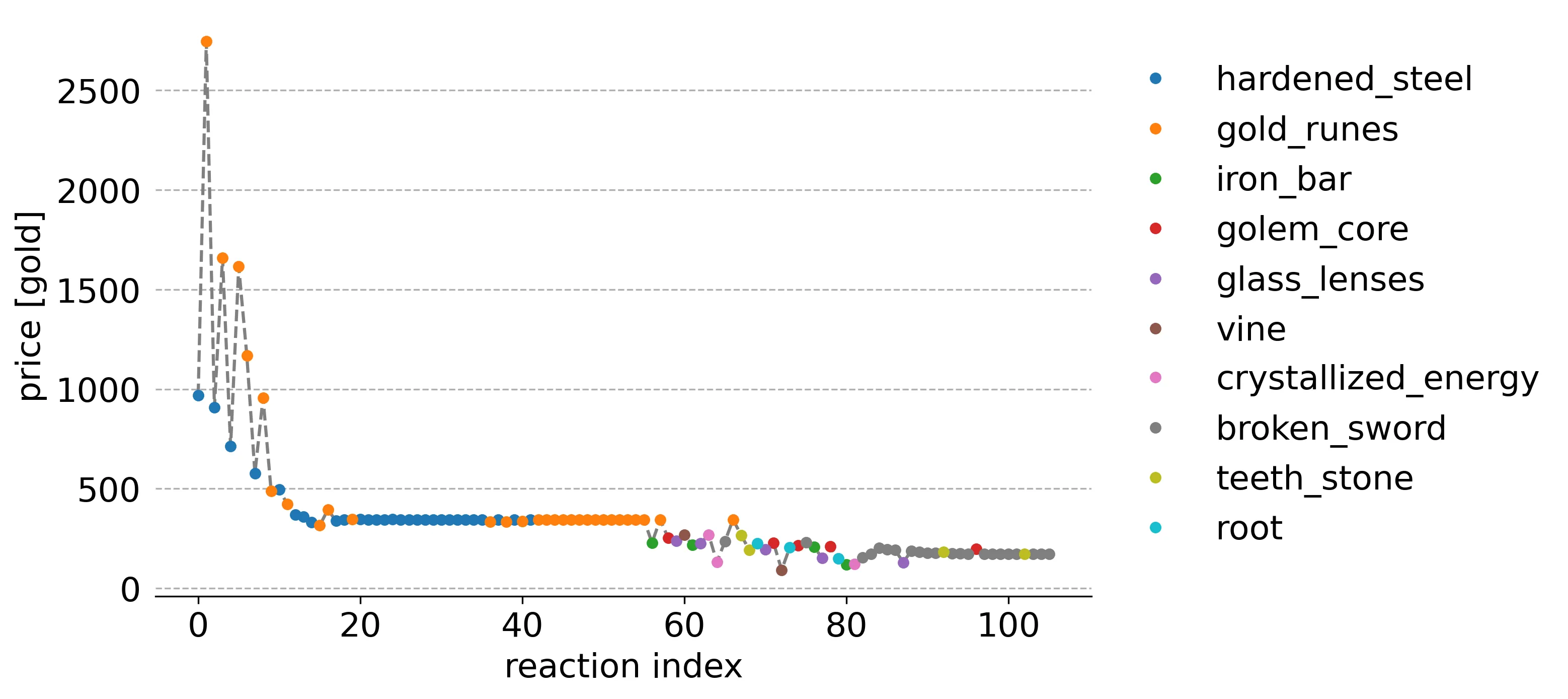
This graph gives us an idea as to what items and prices were being chosen by the algorithm as the simulation progressed. The color of the dot represents what item was present on the shelf the customer randomly selected and the y-axis is the price.

As we saw in the inventory item counts graph, the algorithm initially focused on exploring customer reactions to prices for gold runes and hardened steel. This makes sense since the ledger bounds, which are set as the initial item price bounds, indicated their ideal price should be between 275 and 3000 gold, while that of all others should be between 2 and 275. It then explored price reactions for the remaining items until settling on the broken sword item, corresponding to the second highest ideal price.

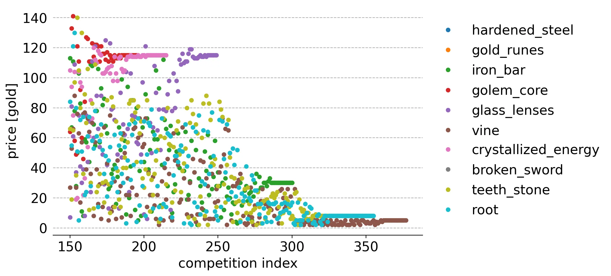
Here's a slightly different view. This is the value of every sampled price for every Thompson sampling competition, from the 10th to the 150th:

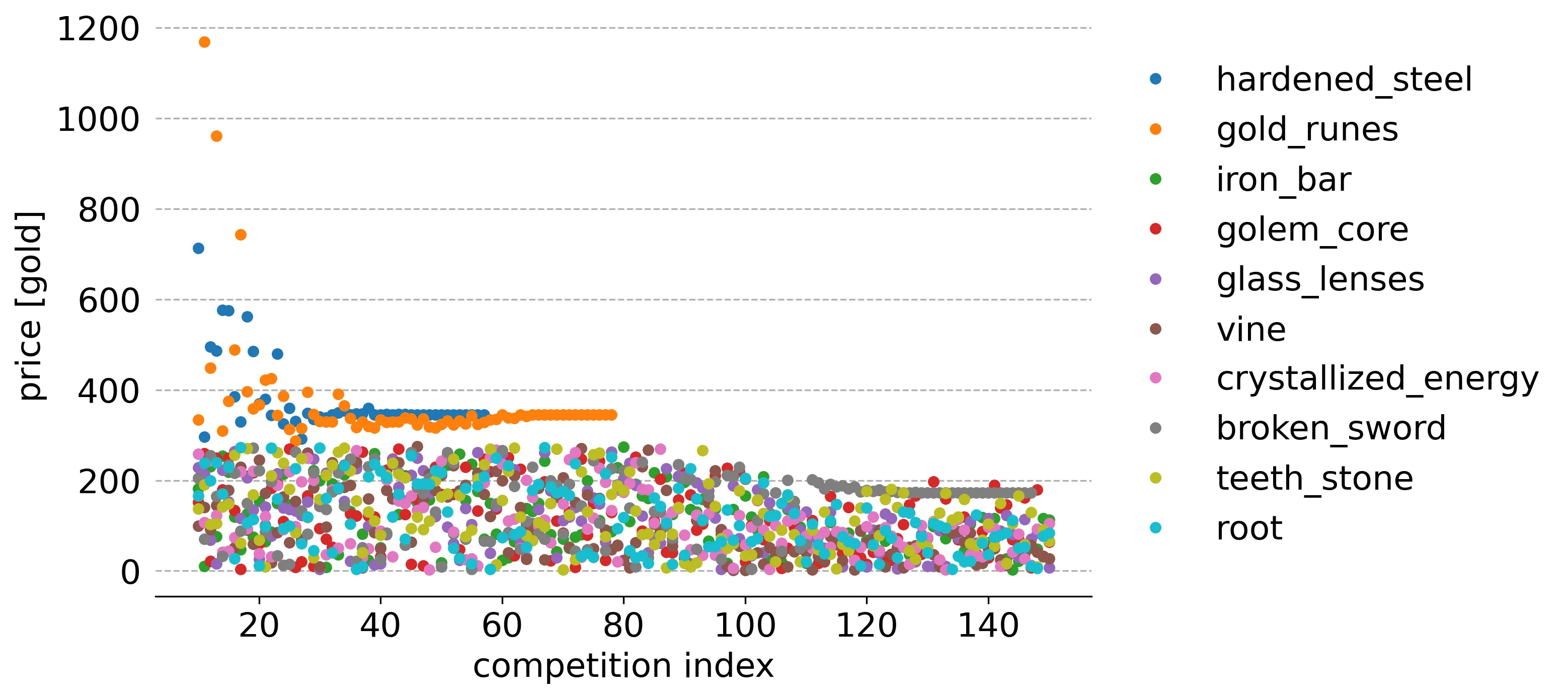
I started from the 10th competition because the scale of the initial points was so high it obscured details I wanted to point out.

Each column of points, at a particular x-value, is a competition between the prices sampled from every item price bound. The highest dot at each step is the item/price that ended up on a shelf. Recall that customer reactions to an item and its price on a shelf cause it to be replaced with a new item and price, determined by Thompson sampling. Additionally, other shelf items can be replaced if their price violates the new bounds resulting from the previous reaction. Note that there are extra steps here, relative to the above customer reaction graph, due to the price bound violations.

Notice how gold runes and hardened steel are the only ones that seem to have the highest price in each step until they are all sold off. Since these are the only items placed on shelves, no customer reactions occur for the other items, preventing their price bound updates. Their sampled prices continue to randomly oscillate between their original ledger bounds until the first two items are exhausted, after which their sampled prices slowly decrease.

Recall that the first two item's ledger bounds are 275 to 3000 gold and that for the other items is 2 to 275. So there IS a remote chance that other items could be selected until the lower bounds for the first two items are raised in response to customer reactions. This would require the sampled price of gold runes, hardened steel, AND one or more of the other items to be 275 and for one of those other items to be randomly selected by the algorithm.

Here's the remaining items and prices resulting from reactions:

After the broken sword inventory was exhausted, the algorithm further explored prices until the third highest ideal price group (i.e. golem core, crystallized energy, and glass lenses) was sold off.

The Bayesian bandits algorithm further explored the prices of remaining items (roughly steps 200 - 212) until selling off iron bars, then the teeth stone and root group, and finally all vines.

Here's the remaining competitions roughly corresponding to the last plot:

There's a pattern where, after some exploration, eventually the algorithm settles on selling only an item or group of items with the same ideal price.

Here I've zoomed in on the Thompson competitions between the teeth stone, root, and vine items in steps 290 to 380 and included ideal price upper and lower bound lines:

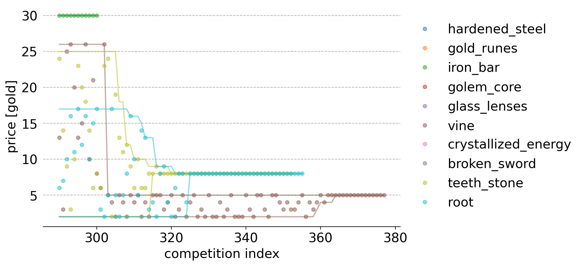
A customer reaction to a vine (brown) item on a shelf, around step 305 or so, results in the algorithm's understanding of its ideal price range to lower so much that it is no longer chosen until teeth stone and root items are sold off.

Somewhere around step 315, the bounds for teeth stone (gold) shrink to very near the ideal price, causing it to be much more likely to be chosen. This is because the sampled price for the root (cyan) item is more likely to be lower, since much of its bounds range is lower than that for teeth stone. Around step 324 the bounds for both teeth stone and root converge to the ideal price and they are randomly selected until both are completely sold off.

Afterwards, the algorithm is able to explore sufficiently to pin down the ideal price of vine and sell it off.

To illustrate some final points, here are a few plots from the perspective of how each reaction affects the algorithm's ideal price bound understanding:

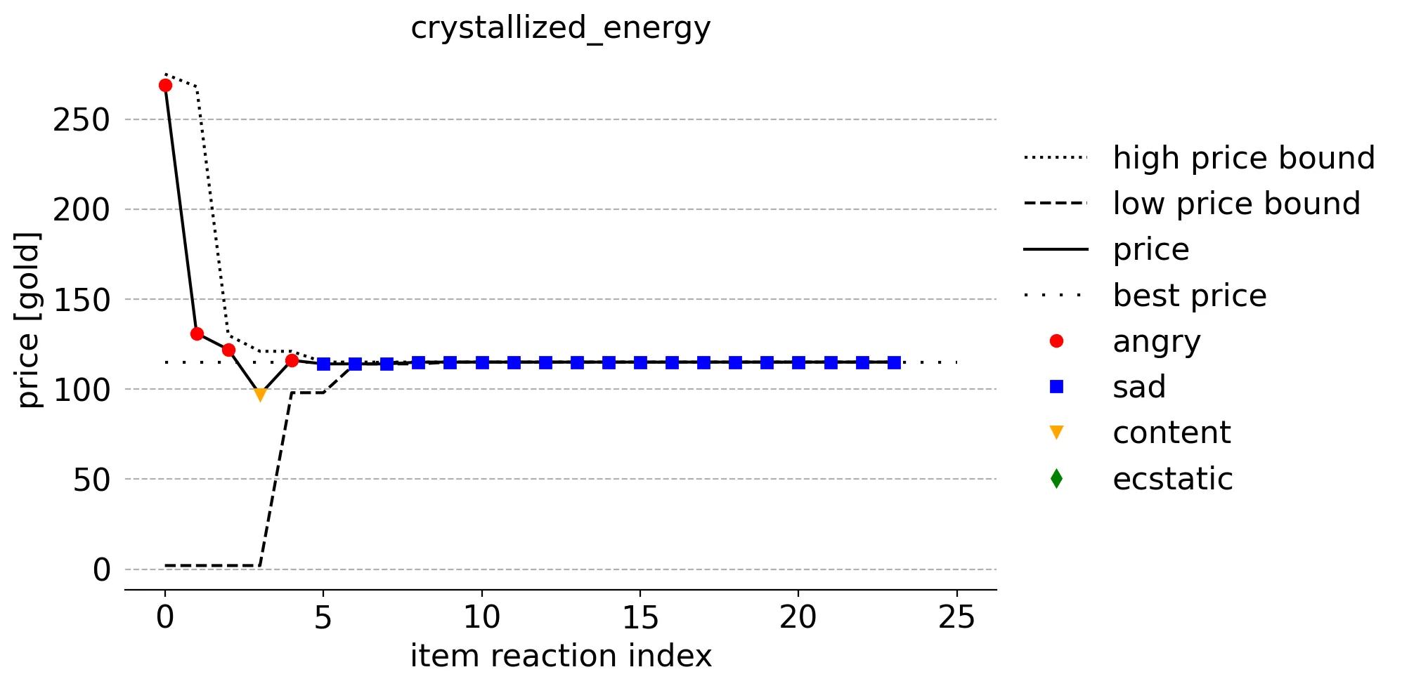
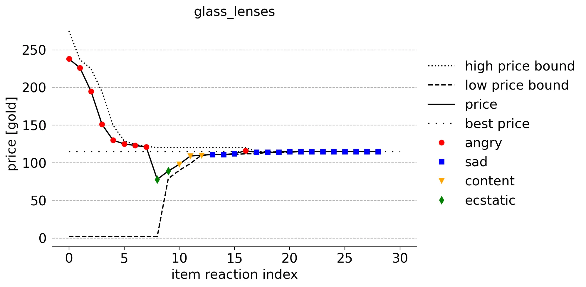
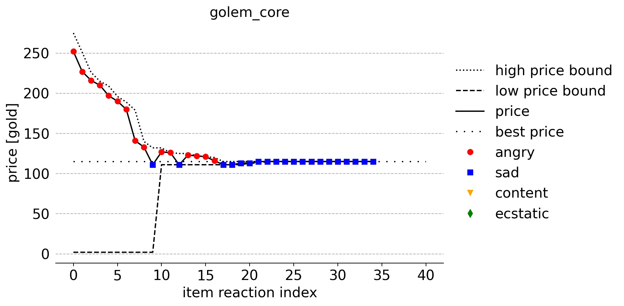
These item-specific plots combine the price on the shelf and corresponding customer reaction mood, the upper and lower ideal price bounds BEFORE the reaction, and the ideal price. The color and shape of the points represent whether the reaction is angry (red circle), sad (blue square), content (orange triangle), or ecstatic (green diamond). For instance, the 4th reaction (reaction index 3) of a customer to a crystallized energy item on a shelf priced just below 100 gold was content (orange triangle).

Notice how angry reactions modify the upper bound after them and how other moods modify the lower bound.

One thing that stands out from these plots, and all of the others like them (not shown), is that the prices tend to start and stay fairly high. Items that end up on a shelf tend to have higher prices since that higher price was necessary to outcompete those sampled from the ideal price distributions. This, of course, ends up making most customers angry and sad. In this context, you could think of this as a happiness minimization algorithm!

The remaining graphs are in the accompanying Jupyter notebook.

Overall, I'm happy with the results from the simulation. Ways to extend this work include:

• Understanding exactly how popularity is set and, maybe, actually building that neat htmx pricing app
• Multiple randomized runs and accompanying statistics to quantify overall behavior
• Comparison to other algorithms like random and/or binary search and/or reinforcement learning agents

Conclusion

I implemented the Bayesian bandits algorithm to price items in a limited simulation of Moonlighter's shop mechanic. The algorithm successfully identified the maximum price customers were willing to pay for each item and sold them in that order, thereby increasing short-term revenue and maximizing customer sadness.

I hope you enjoyed reading this article!

For other applications of Bayesian methods, check out my analysis of data I manually collected in Stardew Valley to figure out optimal crops to plant to maximize revenue or the description of my app to find the Zonai dispensers in The Legend of Zelda: Tears of the Kingdom with the highest probabilities of producing the devices users want.